Getting Started with McRadar

Inside python

First load the package

>>> import mcradar as mcr

Using the mcr object you can verify the default settings

>>> help(mcr.loadSettings)

you will get the following

loadSettings(dataPath=None, elv=90, nfft=512, maxVel=3, minVel=-3,
             ndgsVal=30, freq=array([9.5e+09, 3.5e+10, 9.5e+10]),
             maxHeight=5500, minHeight=0, heightRes=50)

This function defines the settings for starting the
calculation.

Parameters
----------
dataPath: path to the output from McSnow (mandaroty)
elv: radar elevation (default = 90) [°]
nfft: number of fourier decomposition (default = 512)
maxVel: maximum fall velocity (default = 3) [m/s]
minVel: minimum fall velocity (default = -3) [m/s]
ndgsVal: number of division points used to integrate over the particle surface (default = 30)
freq: radar frequency (default = 9.5e9, 35e9, 95e9) [Hz]
maxHeight: maximum height (default = 5500) [m]
minHeight: minimun height (default = 0) [m]
heightRes: resolution of the height bins (default = 50) [m]

Returns
-------
dicSettings: dictionary with all parameters
for starting the caculations

dataPath is the only required parameter. If you try to execute the mcr.loadSettings() without passing a dataPath parameter

>>> mcr.loadSettings()

you will get a warning message

please load the path to the McSnow output
use the dataPath parameter for it
e.g. loadSettings(dataPath="/data/path/...")

Usage Example

The following example computes the spectra and the KDP for a W-band radar with 30° elevation. The data for this example is available here, and inside of the tests folder.

Lets first define the initial settings

>>> dicSettings = mcr.loadSettings(dataPath='data_test.dat', elv=30, freq=np.array([95e9]))

Loading the McTable output

>>> mcTable = mcr.getMcSnowTable(dicSettings['dataPath'])

Selecting a defined time step (e.g. 600)

>>> selTime = 600.
>>> times = mcTable['time']
>>> mcTable = mcTable[times==selTime]
>>> mcTable = mcTable.sort_values('sHeight')

Calculating the spectra and KDP

>>> output = mcr.fullRadar(dicSettings, mcTable)

Congratulations!! You completed all the steps. The output is a xarray dataset, and it allows you to use all the functionalities of xarray of datasets. For example, you can easily save the output and plot the data.

Exporting the output to NetCDF

>>> output.to_netcdf('output.nc')

Note

The plotting functionality is available if you have the matplotlib installed.

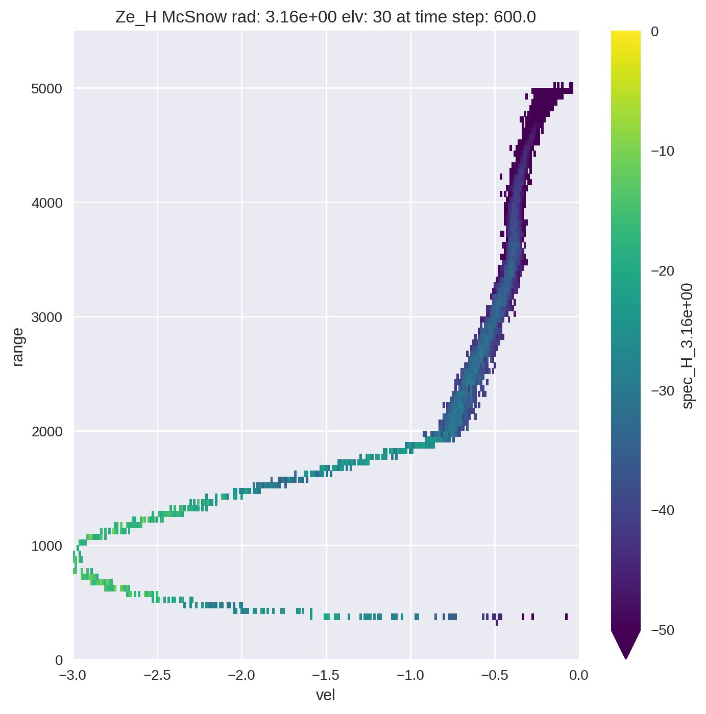
Plotting the spectra

>>> for wl in dicSettings['wl']:

>>>     wlStr = '{:.2e}'.format(wl)
>>>     plt.figure(figsize=(8,8))
>>>     mcr.lin2db(output['spec_H_{0}'.format(wlStr)]).plot(vmin=-50, vmax=0)
>>>     plt.title('Ze_H McSnow rad: {0} elv: {1} at time step: {2}'.format(wlStr, dicSettings['elv'], selTime))
>>>     plt.ylim(dicSettings['minHeight'], dicSettings['maxHeight'])
>>>     plt.xlim(-3, 0)
>>>     plt.grid(b=True)
>>>     plt.show()

You should get the following image